In This Section
Reanalysis Data
Reanalysis data are extensively used in atmospheric science. Briefly, and in order to obtain a first general idea, reanalysis involves analysing past observational data again. These historical observational data are available from different sources such as buoys, radiosondes, ships, meteorological stations or satellites.
They are used to feed numerical weather prediction models through different advanced methods of assimilation, and so transforming an irregularly distributed network of observations into a three-dimensional grid (Bengtsson et al., 2004) of the best estimate of the state of the atmosphere for any period and place (Thorne and Vose, 2010), at different vertical layers of the atmosphere and time steps.
First of all observations are needed. Observational data are employed in model weather forecasts in order to provide the best description possible of the state of the atmosphere at an initial moment. This requires a careful process to recover data and to carry out quality control before data can be used. For example, meteorological stations may be subject to changes in instrumentation, methods of measurement, personnel in charge, changes in location or in the environment of the station such as the effect of urbanisation. However, the station records should ideally reflect only the variation of the weather and climate.
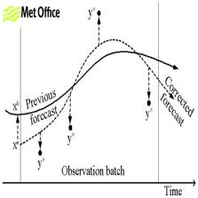
Figure 1. Correction of the model with the observations introduced by assimilation. Source: Met Office.
Furthermore, the available observational data change qualitatively and quantitatively between countries and inside them, along with changes over the periods they are recorded and in their spatial distribution. Since 1979 the use of weather satellites has allowed more data to be incorporated in the assimilation process. If the observational systems, the model or the method of assimilation are improved, the new reanalysis data obtained corresponds to a new generation. That way it is possible to distinguish between 1st generation reanalysis data such as NCEP/NCAR (National Center for Environmental Prediction / National Center for Atmospheric Research), 2nd generation such as ERA40 data from the ECMWF (European Centre for Medium-Range Weather Forecasts) and 3rd generation like the MERRA (Retrospective analysis for Research and Applications). The ERA-40 was surpassed by the ERA-Interim data (3rd generation) and currently, by the recently launched ERA5 (4th generation reanalysis). Each generation implies an improvement in the data used to characterise the state of the atmosphere.
The incorporation of observations into the model is done by a process called assimilation. The observations are introduced at different times to correct the model in order to ensure that the evolution of the atmosphere during the simulation is as close as possible to the real observed conditions of the atmosphere. The initial forecast created by the model is corrected with the observational data during the execution of the model (figure 1). The output of the model is fitted to those observations to obtain a corrected forecast.
The observations can be introduced into the model at different stages while the model is running, by “running” we mean while the model is executing all the instructions that we have given to it. It can be thought of as similar to the calculations performed by a calculator after typing in “2+2” and before the result of 4 is displayed. Aside from observations, the forecast obtained in the previous time step by the model is used as input in the following time step analysis.
There are different types of assimilation (figure 2).
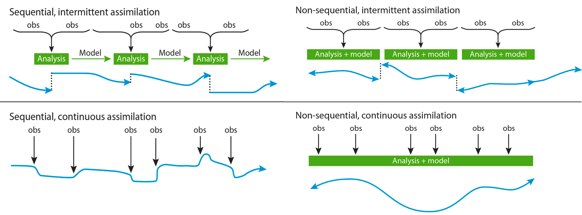
Figure 2. Methods for the reanalysis data assimilation process. Source: National Center for Atmospheric Research.
The assimilation is intermittent when the available observations over a range of time are introduced at regular intervals into the model. On the other hand, if the assimilation is continuous, every time there is an observation, it is introduced into the model at the time when the observation was registered.
In the sequential assimilation method the simulation is always in a forward direction, using the corrected outputs of the model in each stage as input for the next forecast or using only observations as inputs. In any case, the assimilation is done in the same direction in time. However, if the method is non-sequential, at each step of the model or at the end of the simulation, the corrected output constitutes again an input at the beginning of each time step or at the very beginning of the simulation.
When the available observations are scarce, the model accuracy is low, and the output of the model reflects mainly the variability of the model being used. If we increase the observations, the model is forced to follow the observations (Sterl, 2004). So, the more observations we have, the less important the model becomes. In any case, we would still have different sources of uncertainty or errors, such as the quality of the observations, the method of assimilation or the particular model used and its characteristics such as the parameterisations chosen.
Numerical Weather Prediction (NWP) models are physico-mathematical models used to reproduce the evolution of the atmosphere over time. NWP models calculate the state of the atmosphere at discrete locations in a three-dimensional grid. Some of the meteorological processes and phenomena in the atmosphere take place in a lower spatial resolution than the size of NWP models’ grid cells, for example convection or cloud microphysics. The NWP models use parameterisations to reproduce the dynamic and thermodynamic conditions for these phenomena to occur. They can be thought as formulae that use the information available at a coarse resolution to try to reproduce those phenomena at a finer resolution.
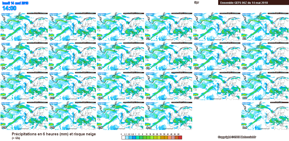
Figure 3. Ensemble members (from P1 to P20 (perturbation)) of the NWP model GEFS (Global Ensemble Forecast System). Forecast of precipitation made at 06UTC on the 14th May 2018, for the same day at 14:00 UTC. Source: Meteociel.
The model can be run several times to obtain different possible solutions to the meteorological evolution of the atmosphere. The group of all those outputs is called ensemble (figure 3). This way it is possible to take into account the chaotic nature of the atmosphere and the uncertainty of the initial state of the atmosphere.
Another way to visualise the ensembles is through diagrams (figure 4). The uncertainty of the forecast increases with time, as is indicated by the increasing spread of the ensembles.
Figure 4. Diagram of ensembles for a point in the south of Ireland (coordinates 51.9N and 8.9W). From top to bottom, ensembles for the temperature at 850 hPa and at 500 hPa, and precipitation.
Reanalysis data offer valuable information about the atmospheric conditions necessary or favourable for a particular phenomenon to happen, for example, to determine the position of the jet stream or the location of low and high pressure systems. Reanalysis data can also be employed for the study of trends or in attribution studies.
Given the disparity in the availability of observational data, is not uncommon that there is no such data available for use in climatological studies due to a low spatial and/or temporal resolution. Moreover, when dealing with extreme weather and climate events, which by definition are rare at any point, it is even more difficult to collate long and homogeneous records from observational data. Reanalysis data also offer the possibility to construct proxies for parameters or indices that could be used to characterise, either from the thermodynamic or the dynamic point of view, the event being studied in the case of that a useful direct output from the model is not available.
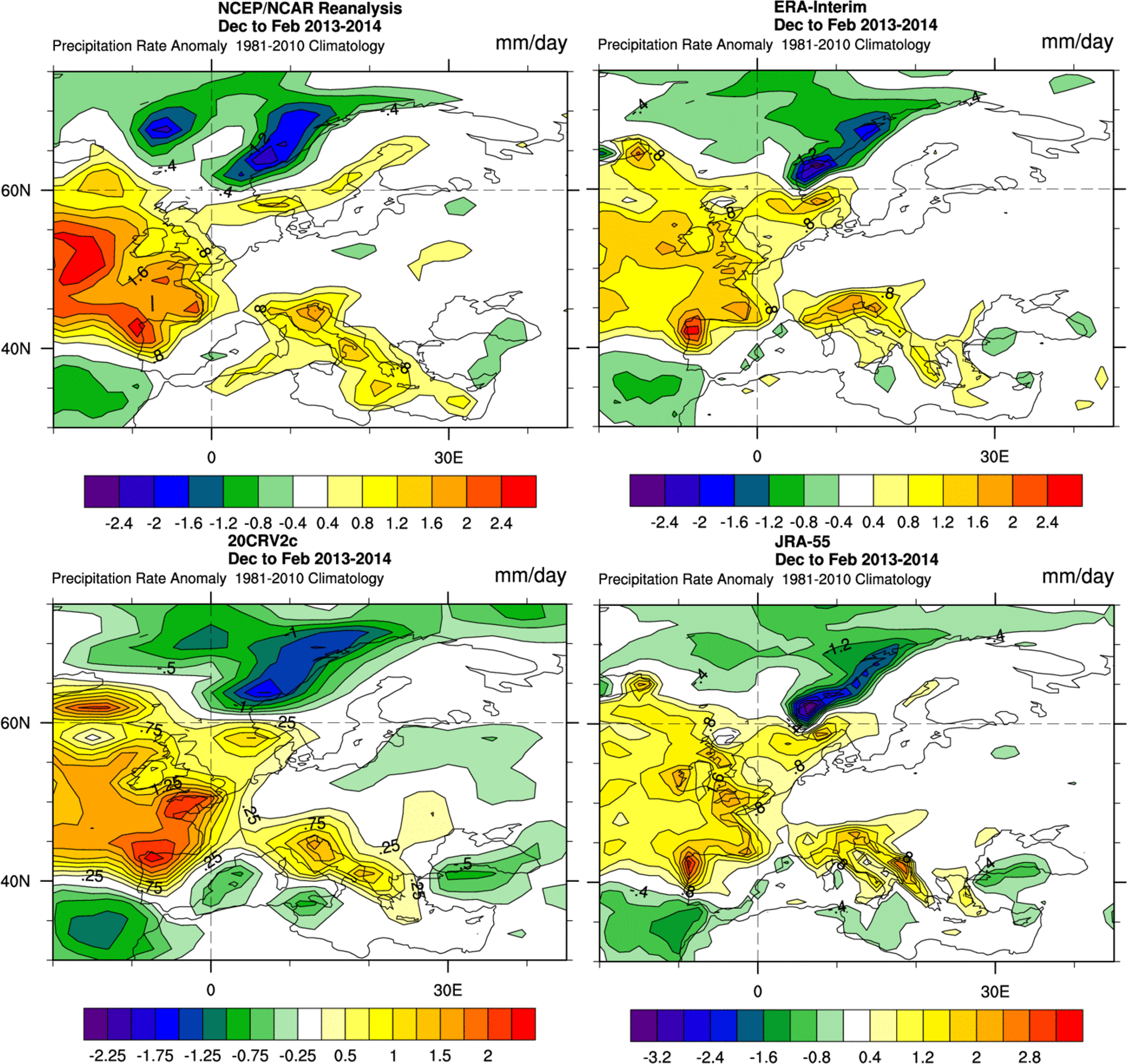
Figure 5. Precipitation anomaly (mm/day) in winter 2013/2014 respect to the period of reference 1981-2010. Output from four different reanalysis data: NCEP/NCAR, ERA-Interim, 20CRV2c and JRA-55. Maps created with the online tool: https://www.esrl.noaa.gov/psd/cgi-bin/data/testdap/plot.comp.pl.
When using reanalysis data is important to choose the best option for the objective of our study (figure 5 and 6). Different datasets are based on different historical observational data, number of vertical levels or different temporal and spatial resolution, among other factors.
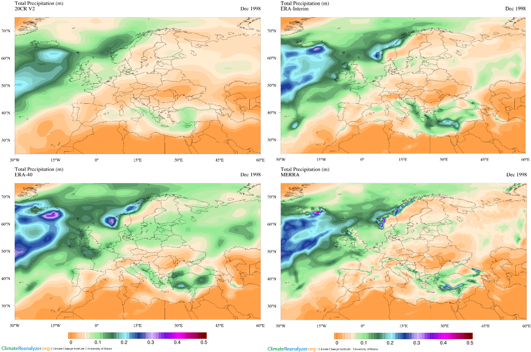
Figure 6. Precipitation anomaly (mm/day) in winter 2013/2014 respect to the period of reference 1981-2010. Output from four different reanalysis data: NCEP/NCAR, ERA-Interim, 20CRV2c and JRA-55. Maps created with the online tool: http://cci-reanalyzer.org/
Met Éireann, the Irish Meteorological service, has launched a specific reanalysis product for Ireland called MÉRA. These data have an excellent horizontal resolution of 2.5 km and go back to 1981.
So, what are you waiting for to start working with reanalysis data? Do you want to explore the possibilities to complement your research results? You can become familiar with this kind of data by using very simple web-based tools to plot the data of your interest.
REFERENCES
- Bengtsson, L., Hagemann, S. and Hodges, K.I. (2004). Can climate trends be calculated from reanalysis data? Journal of Geophysical Research: Atmospheres, 109(D11).
- National Center for Atmospheric Research Staff (Eds). (Last modified 20 Aug 2013). “The Climate Data Guide: Simplistic Overview of Reanalysis Data Assimilation Methods. [Accessed 17th Oct. 2017].
- Sterl, A. (2004). On the (in) homogeneity of reanalysis products. Journal of Climate, 17(19), pp.3866-3873.
- Thorne, P.W. and Vose, R.S. (2010). Reanalyses suitable for characterizing long-term trends. Bulletin of the American Meteorological Society, 91(3), pp.353-362.
ClimATT
Climate Change Attribution of Extreme Weather Events
Contact us